Chapter 27 The t test
#Set a range of x values
x.values <- seq(-4,4,0.01)

#Plot a  distribution of t values with 3 degrees of freedom for the corresponding x values
plot(x.values,dt(x.values, 3), type="l", lty=1, lwd=2, ylim=c(0,0.4), xlab="t or Z", ylab="probability")

#Plot a normal distribution over the t distribution
lines(x.values, dnorm(x.values), type="l", lty=2, lwd=2, col="red")

#add lines that define the 5% critical values for the normal distribution
abline(v=qnorm(c(0.025,0.975)), col="red")

#add lines that define the 5% critical values for the t distribution with 3 degrees of freedom
abline(v=qt(c(0.025,0.975),3), col="black")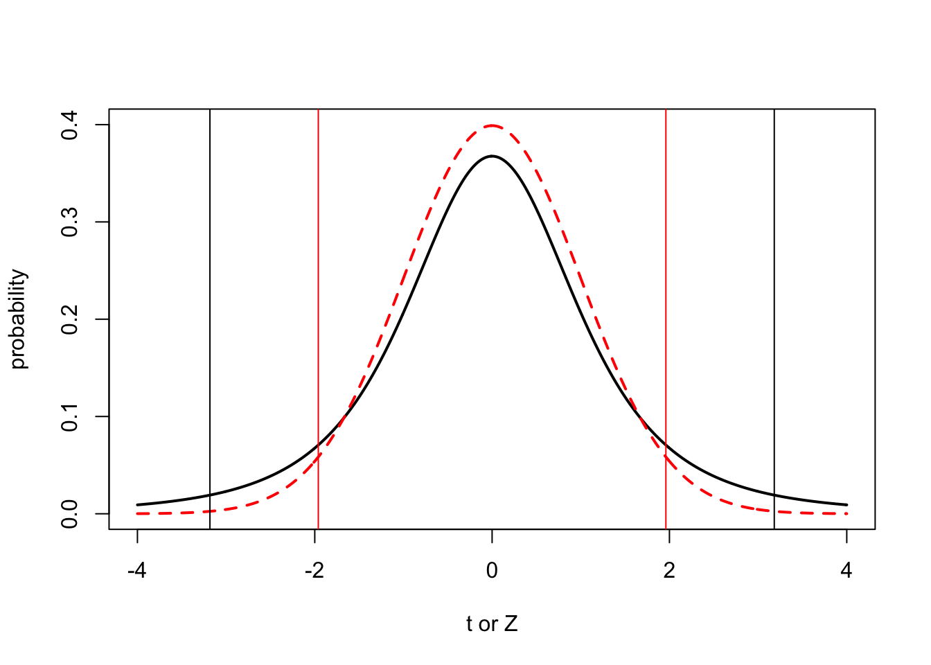
#Draw the t-distribution with 5% critical values colored in
plot(x.values,dt(x.values, 3), type="l", lty=1, lwd=2, ylim=c(0,0.4), xlab="t", ylab="probability")
xvals <- seq(-4,qt(0.025,3),length=50)
dvals <- dt(xvals,3)
polygon(c(xvals,rev(xvals)),c(rep(0,50),rev(dvals)), col=5)

xvals <- seq(qt(0.975,3),4,length=50)
dvals <- dt(xvals,3)
polygon(c(xvals,rev(xvals)),c(rep(0,50),rev(dvals)), col=5)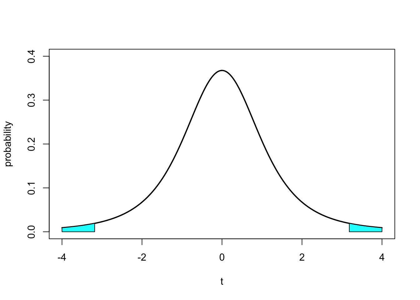
## [1] 3083.732## [1] 548.0283#take a random sample of 9 values and print out the mean and standard deviation
r <- sample(BirthWeight$Weight, 9)
mean(r)## [1] 3515.222## [1] 375.585827.1 One sample t test
#Generate the "Bigbaby" birthweights by artificially inflating the sampled birthweights
bb <- sample(BirthWeight$Weight, 13)*1.5
mean(bb)
## [1] 4730.077## [1] 807.464## [1] 223.9502#calculate the t test statistic without using the inbuilt function in R
t.stat <- (mean(bb)-3048)/(sd(bb)/sqrt(13))
1-pt(t.stat,12)## [1] 3.564286e-06#one sample t-test to test whether birth weight of babies born to mothers with the "C" allele of the Bigbaby gene are different from the
#average birthweight of 3048 grams
t.test(bb, mu=3048, alternative = "greater")##
## One Sample t-test
##
## data: bb
## t = 7.5109, df = 12, p-value = 3.564e-06
## alternative hypothesis: true mean is greater than 3048
## 95 percent confidence interval:
## 4330.933 Inf
## sample estimates:
## mean of x
## 4730.07727.2 Exploring T-tests
Ho: the true mean of babies born to mothers carrying the BigBaby “G” SNP is 3048 (the average birthweight of all children)
Ha: the true mean of babies born to mothers carrying the BigBaby “G” SNP is greater than 3048
#Plot a population sample of all birthweights
xv <- seq(312,6492,1)
#multiply by total sample size (54345) and bin size (250) so that distribution looks like the frequency distribution of all birthweights
yv <- dnorm(xv,mean=3048,sd=548)*53435*250
plot(xv,yv, lwd=6, type="l", xlab="birthweight (grams)", ylab="frequency")
abline(v=3048)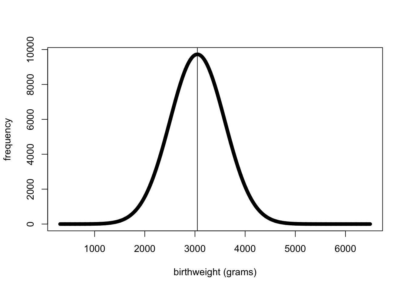
##Plot a population sample of nicebaby G SNP birthweights
#multiply by total sample size (534) and bin size (250) so that distribution can be compared to the previous plot (i.e. the frequency of each bin is 10-fold less)
yv <- dnorm(xv,mean=3048,sd=548)*534*250
plot(xv,yv, lwd=6, type="l", xlab="birthweight (grams)", ylab="frequency")
abline(v=3048)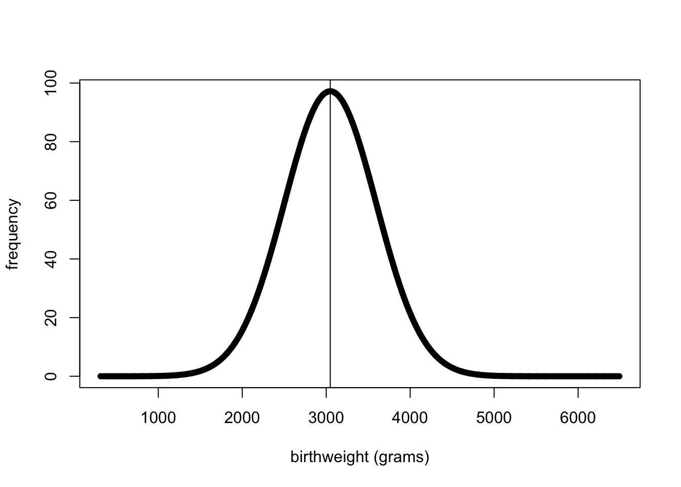
#take a random sample of 5 birthweights from the nicebaby G SNP birthweights.  In reality this is all we are typically able to see.
sample1 <- sample(rnorm(5, mean=3048, s=548))
hist(sample1, main = "n=5", xlim=c(500,6500), ylim=c(0,1.5), br=6000, col="blue", lty=2)
abline(v=mean(sample1), col="red")
print(mean(sample1))
## [1] 2695.625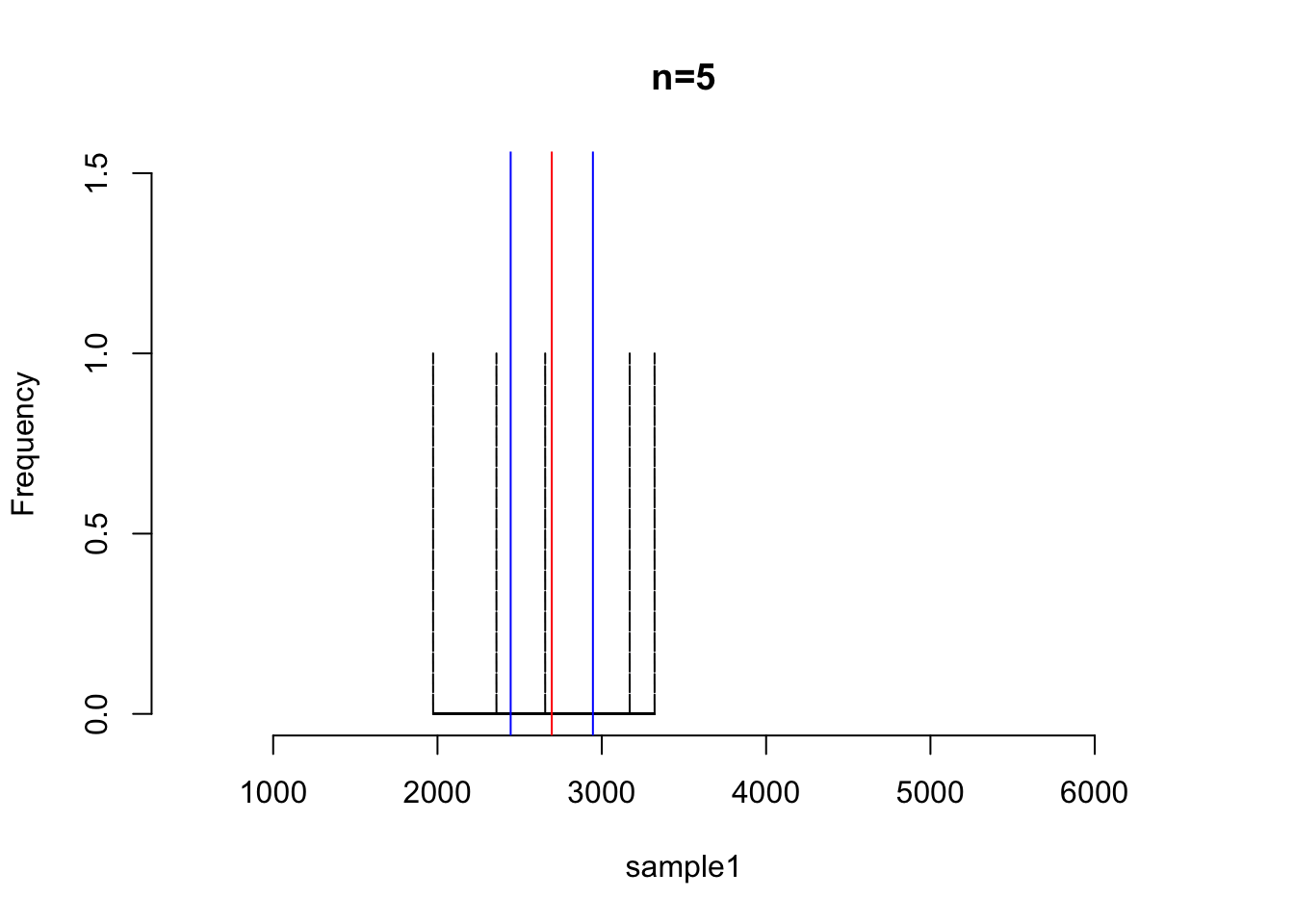
s.e.1 <- sd(sample1)/sqrt(5)

#take another random sample of 5 birthweights from the nicebaby G SNP birthweights.  The important point here is taht the sample is different and so is the sample mean and the standard error
sample2 <- sample(rnorm(5, mean=3048, s=548))
hist(sample2, main = "n=5", xlim=c(500,6500), ylim=c(0,1.5), br=6000, col="blue", lty=2)
abline(v=mean(sample2), col="red")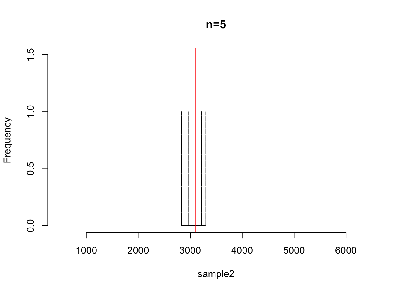
## [1] 3106.719s.e.2 <- sd(sample2)/sqrt(5)
#compute sampling distribution of the mean for n=5. That is take random samples of size 5 and compute the sample mean.
sample.means <- numeric(10000)
for(i in 1:10000) {
sample.means[i] <- mean(sample(rnorm(5, mean=3048, s=548)))
}
#Plot the distribution of sample means. This is the sampling distribution of means
hist(sample.means, col="green", xlim=c(500,6500), main="Distribution of sample means, n=5")
abline(v=mean(sample.means), col="red", lwd=4)
#Add lines that indicate one (blue) and two (black) standard deviation of the distribution of means (this is the standard error of the mean)
abline(v=c(mean(sample.means)-sd(sample.means),mean(sample.means)+sd(sample.means)), col="blue", lwd=4)
abline(v=c(mean(sample.means)-2*sd(sample.means),mean(sample.means)+2*sd(sample.means)), col="black", lwd=4)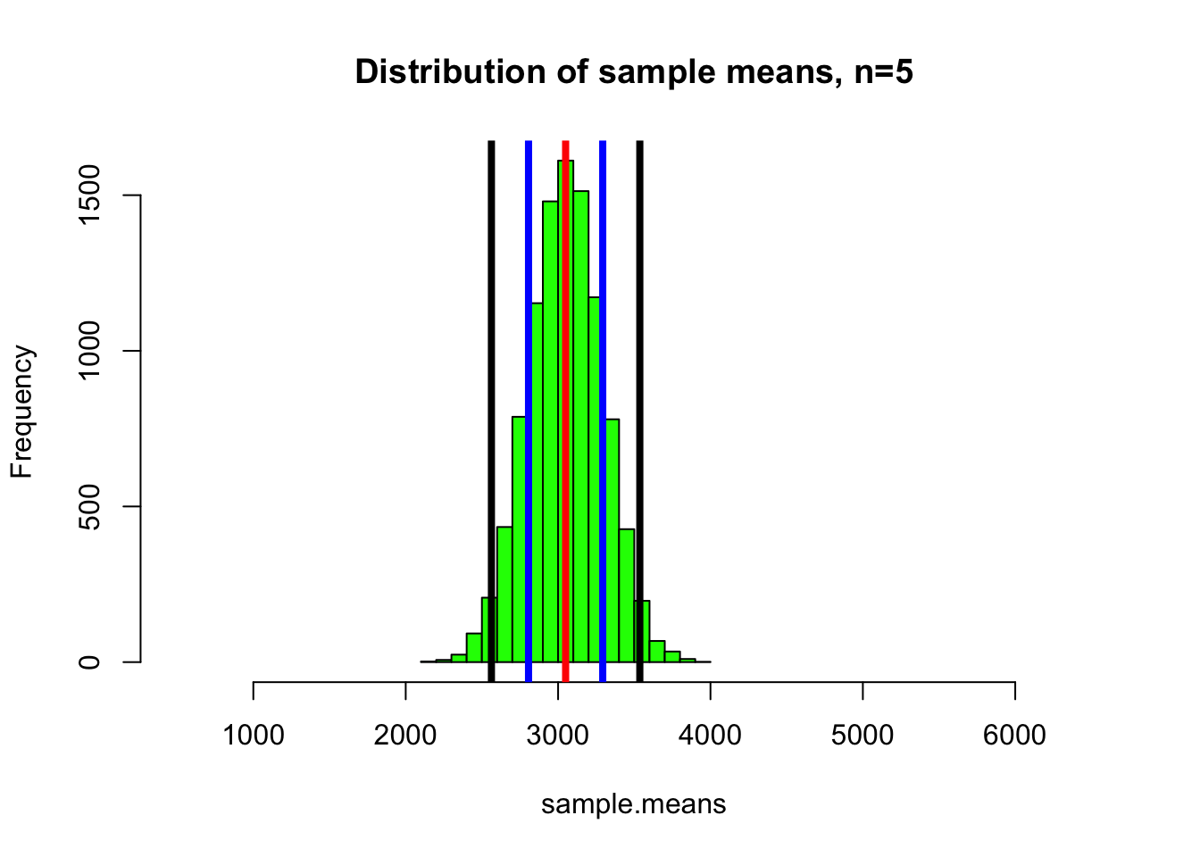
#the standard deviation of the sample distribution can also be calulated by dividing the population standard deviation (which we've set to 548) by sqrt(sample size)
print(sd(sample.means))
## [1] 243.4492## [1] 245.073127.3 Produce the null distribution of the t statistic by simulation
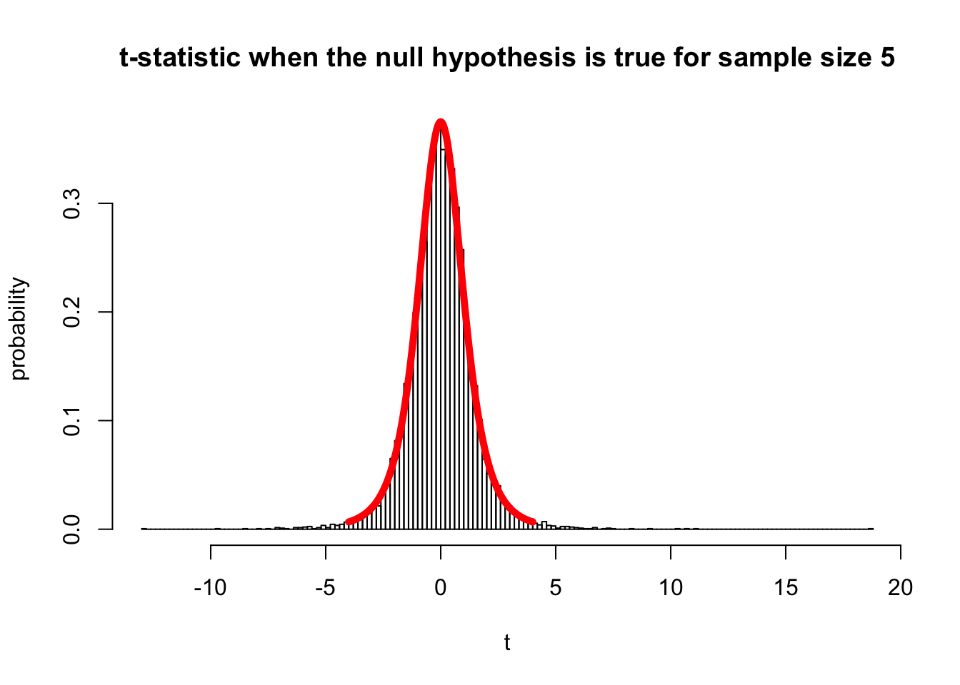
To do this we will randomly sample from a normal distribution with sample size 5 and compute the t test statistic for each random sample. Plot the empirical distribution of 2 values
a <- numeric(10000)
for(i in 1:10000) {
sampleA <- rnorm(5, mean=3048, s=548)
a[i] <- t.test(sampleA, mu=3048)$statistic
}

hist(a, br=200, freq=F, ylab="probability", xlab="t", main="t-statistic when the null hypothesis is true for sample size 5")

#Superimpose the  theoretical distribution of t values for 4 degrees of freedom
x.values <- seq(-4,4,0.01)
lines(x.values,dt(x.values, 4), type="l", lty=1, lwd=5, col="red")