Chapter 22 Genetic Drift

In this chapter we will examine the concept of genetic drift.

evo<-function(t,pop,ip){
pplot<-matrix(NA,t,10)
pplot[1,]<-ip

for (i in 1:10){
p<-ip
for (t in 2:t){
x<-rbinom(1,pop,p)
p<-x/pop
pplot[t,i]<-p}}
pplot
}

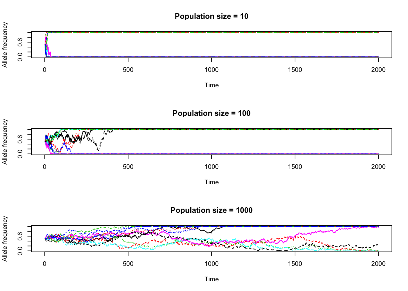
a<-evo(2000,10,0.5)
b<-evo(2000,100,0.5)
c<-evo(2000,1000,0.5)

par(mfrow=c(3,1))
t<-1:2000
matplot(t,a,type='l',main='Population size = 10',xlab='Time',ylab='Allele frequency', ylim=c(0,1))
matplot(t,b,type='l',main='Population size = 100',xlab='Time',ylab='Allele frequency', ylim=c(0,1))
matplot(t,c,type='l',main='Population size = 1000',xlab='Time',ylab='Allele frequency', ylim=c(0,1))