Chapter 6 Sampling from populations
6.1 Sampling from populations
In this chapter, our goal is to learn about the concept of sampling from a large population. We can simulate this process in the computer to understand what is actually happening when we take a small sample from a large population and attempt to make an inference about the entire population.
6.2 Simulating a population of student heights
We want to create a fictional population of heights in a population of students. To do this, we just need to select two summary statistics that characterize a normal distribution - the average height and the standard devaition. We also need to define how many individuals are in our population. So, let’s choose some reasonable values:
- average height = 170cm
- standard deviation = 10cm
- population size = 21,000 individuals
Since we are going to simulate this population in R, we need to make those paramaters variables in R:
The R function rnorm() will generate a simulated population for us with the specified parameters (mean and standard deviation).
You can learn about the function by typing ?rnorm at the command prompt
Now, we can generate our population by specifying those three parameters.
6.2.1 Generate a histogram that summarizes the distribution of heights in the entire population.
We plot the distribution of heights in the entire population using the function hist()
To help in visualization, let’s also add a vertical line indicating the mean height and +/- 1 standard deviation using the function abline()
hist(pop.heights, br=100, main="Distribution of heights in student population", xlab="height (cm)")

abline(v=mean(pop.heights), col="red", lwd=6, lty=2)
abline(v=mean(pop.heights)+sd(pop.heights), col="blue", lwd=3, lty=2)
abline(v=mean(pop.heights)-sd(pop.heights), col="blue", lwd=3, lty=2)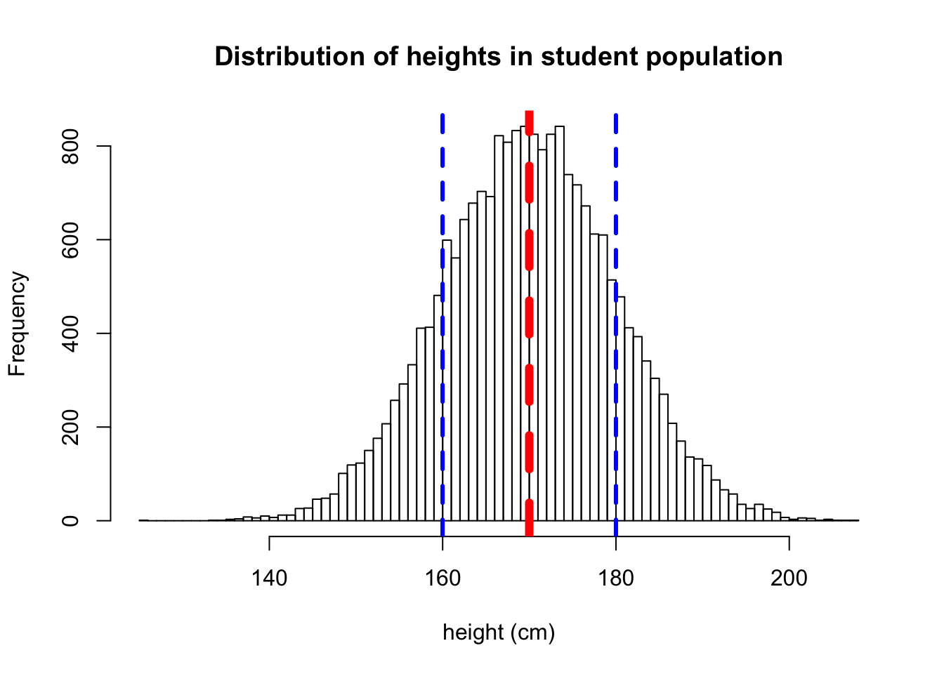
Figure 6.1: Population heights
6.2.2 Simulating the process of sampling from a large population.
In the real world,we are typically not able to measure the heights of all individuals in a population. Instead, a common approach is to take a random sample from the population, and determine the summary statistics of this sample. We then make an inference about the population on the basis of our sample. For example, we can estimate the average population height and the population standard deviation by calculating the average height in the sample and the standard deviation of the sample.
As we can see from the red line in 6.1 the average height in our simulated population is 170cm, which was a populaton parameter that we specified in simulating the population.
Now, we want to simulate the process of sampling from the population. Let’s imagine that we take a sample of 17 individuals. We can simulate the process of sampling 17 individuals from this population using the function sample().
Now let’s plot the FREQUENCY distributiion of our sample of 17 randomly chosen individuals from the population and add a line indicating the mean of our sample.
hist(sample1, main="Frequency distribution of human heights, n=17", xlab="height (cm)")
abline(v=mean(sample1), col="red", lwd=6, lty=2)
Figure 6.2: Sample 1 heights
## [1] "The average height in sample 1 of 17 individuals is: 171.0184112397"In most cases our sample mean is going to differ from the population mean. Therefore, we can think of our sample mean as a random variable.
To illustrate the concept that the sample mean is a random variable, let’s simulate taking a completely different sample of 17 individuals from our population of 20,000 individuals and look at the result.
sample2 <- sample(pop.heights, size=17)
hist(sample1, main="Frequency distribution of human heights, n=17", xlab="height (cm)")
abline(v=mean(sample1), col="red", lwd=6, lty=2)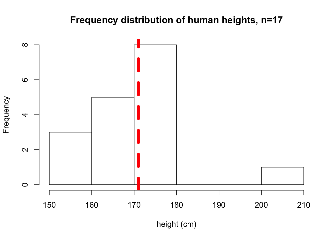
Figure 6.3: Sample 2 heights
## [1] "The average height in sample 2 of 17 individuals is: 168.079783098134"6.3 Repeating the process of sampling over and over
By simulating the process of sampling from a population thousands of times we can obtain the distibrution of sample means. All we need to do to determine the sampling distribution of means is repeat our sampling procedure 10,000 (or more) times and calculate the sample mean each time.
R allows us to do this very easily using a concept in computer programming called a loop.
A loop has two parts:
- We need to define how many times we want to repeat something which we indicate with the synatx:
for(i in 1:10000) - We need to tell R what to do each time we go through the loop. We put this command in curly brackets:
{}
Often, we want to keep a record of what the result was each time we went through the loop. To do that, we define a variable (a vector in this case) in which we can store the information generated in the loop. Initially, the contents of the vector will be empty, which we can see by looking at the first 10 values.
## [1] 0 0 0 0 0 0 0 0 0 0In the loop below I am 1) taking a sample from the population 2) calculating the mean of that sample and recording it.
for(i in 1:10000) {
this.sample <- sample(pop.heights,size=17)
sample.means[i] <- mean(this.sample)
}
Now the variable sample.means should have information in it. Let’s look at the first ten values:
##  [1] 165.9174 168.7802 175.4548 168.8975 168.3814 169.0191 165.1725
##  [8] 169.6101 168.9741 171.3583
Now let’s plot the PROBABILITY distribution of SAMPLE MEANS and indicate the mean of means with a read line.
hist(sample.means, main = "Probability of sample means, n=17", xlab="sample mean height (cm)", xlim=c(160,180))
abline(v=mean(sample.means), col="red", lwd=6, lty=2)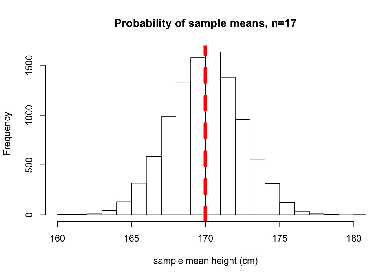
Figure 6.4: Distribution of sample means
This distribution is distribution of sampling means. It is a probability distirbution that defines the chance of getting a specific sample mean value when we take a random sample from our population.
Interestingly, you can see that the mean of the sample means is:
## [1] 169.98296.4 Exercises
- Generate a fictional population of 100,000 blood pressure values for healthy females aged 30-50.
- Construct a histogram with correct axis labels
- Simulate taking sample sizes of 10, 100 and 1000 from the population
- Make a three panel plot in which you plot the distubution of sample means.
- Bonus: determine the mean and standard deviation of each distribution.