Chapter 14 The binomial distribution

The binomial distribution allows us to assess the probability of a specified outcome from a series of trials. Typically, we think of flipping a coin and asking, for example, if we flipped the coin ten times what is the probability of obtaining seven heads and three tails.

The exact same logic can be applied to human inheritance of mendelian traits. For example, we can ask in a family segragating an autosomal dominant disease, what is the probability of having seven affected children and three unaffected children.

14.1 Combinations

Often we don’t care about the specific order of events. In that case we are simply want to ask the case how many different (unique) ways are there of selecting \(x\) successes from \(n\) trials.

To do this in R we use the function choose(). For example, how many different ways are there to choose 1 from 5?

choose(5,1)

## [1] 5

This rapidly increases, for example,how many different ways are there to choose 10 from 500?

choose(500,10)

## [1] 2.458106e+20

14.2 The binomial distribution

Compute the probability of 0-4 affected children given an affected father and autosomal dominant inheritance using the binomial theorem

choose(4,0)*(1/2)^0*(1/2)^4 #0 affected

## [1] 0.0625

choose(4,1)*(1/2)^1*(1/2)^3 #1 affected

## [1] 0.25

choose(4,2)*(1/2)^2*(1/2)^2 #2 affected

## [1] 0.375

choose(4,3)*(1/2)^3*(1/2)^1 #3 affected

## [1] 0.25

choose(4,4)*(1/2)^4*(1/2)^0 #4 affected

## [1] 0.0625

Now let’s plot the probability distribution of 0-4 affected children given an affected father and autosomal dominant inheritance using the binomial theorem

dom.0 <- choose(4,0)*(1/2)^0*(1/2)^4
dom.1 <- choose(4,1)*(1/2)^1*(1/2)^3
dom.2 <- choose(4,2)*(1/2)^2*(1/2)^2 
dom.3 <- choose(4,3)*(1/2)^3*(1/2)^1 
dom.4 <- choose(4,4)*(1/2)^4*(1/2)^0

barplot(c(dom.0,dom.1,dom.2,dom.3,dom.4), names.arg=c(0,1,2,3,4), ylab="probability", xlab= "number of affected children", main = "Probability of affected number of children in a family of four given autosomal dominant inheritance")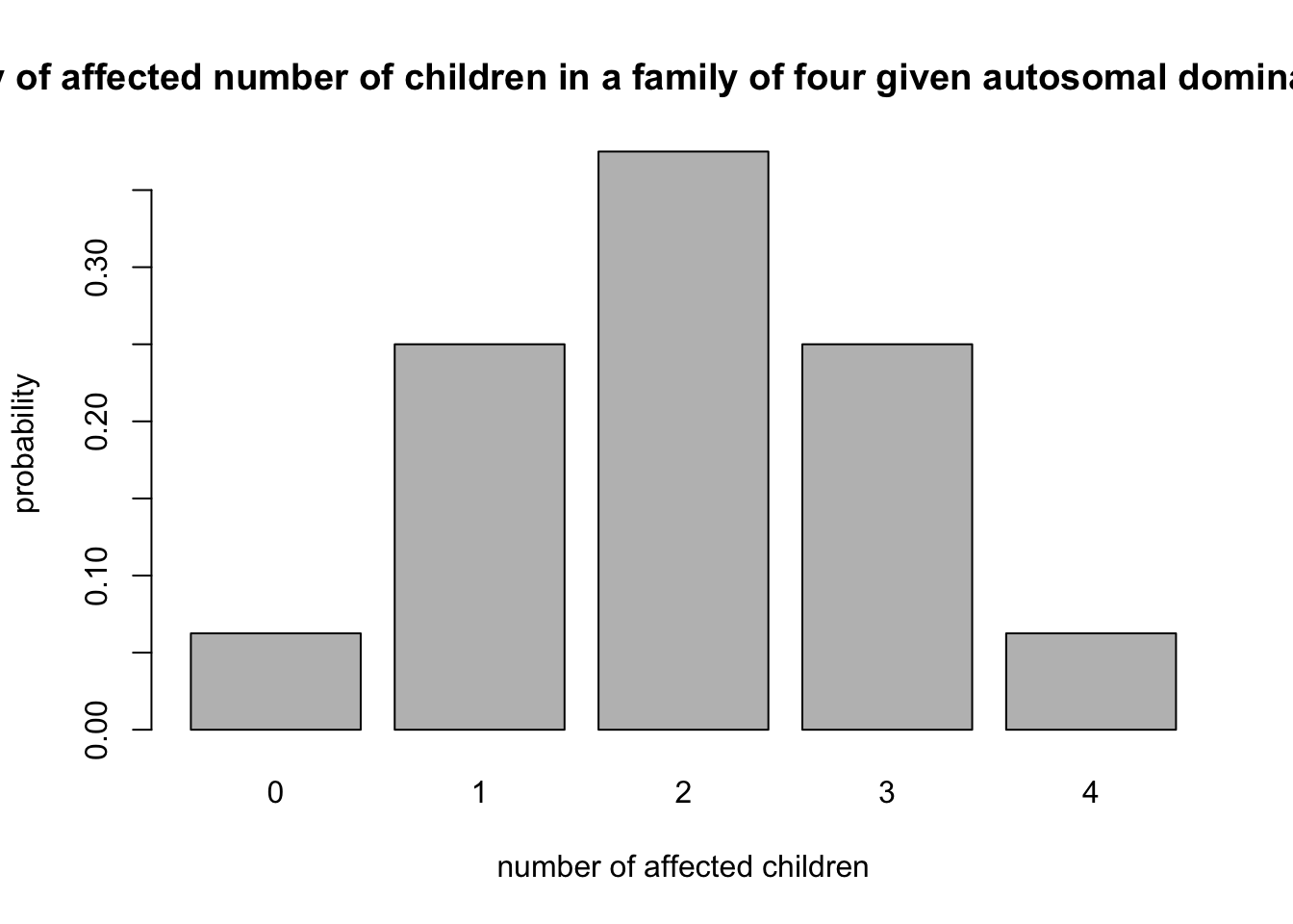

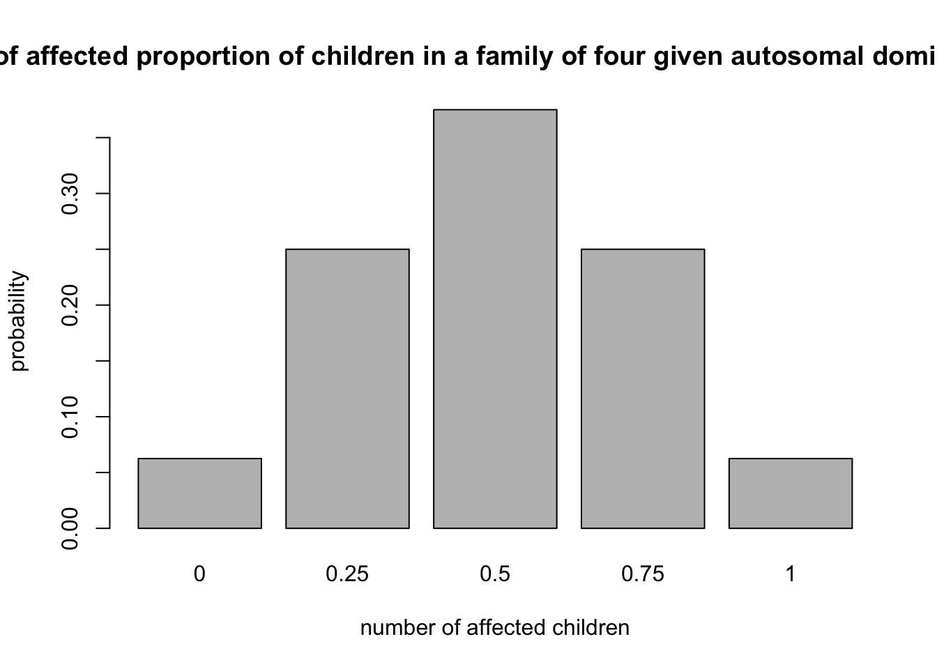
we can make the same plot as a proportion by diving the x-axis values (X) by the total (n)

barplot(c(dom.0,dom.1,dom.2,dom.3,dom.4), names.arg=c(0,1,2,3,4)/4, ylab="probability", xlab= "number of affected children", main = "Probability of affected proportion of children in a family of four given autosomal dominant inheritance")

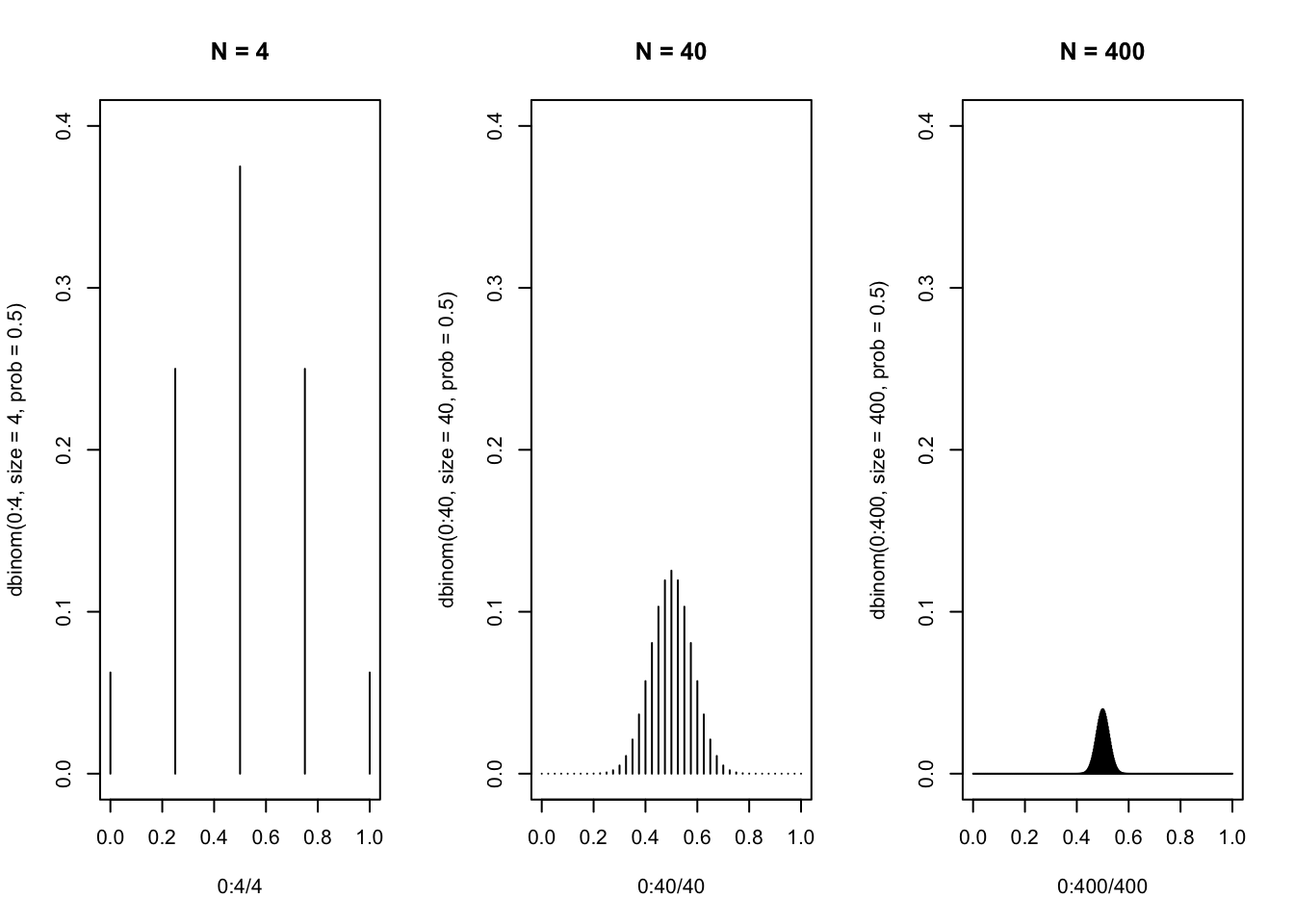
14.3 Binomial probabilities and sample size

Let’s look at how the variance in the binomial distribution changes as the sample size increases?

par(mfrow=c(1,3))

plot(0:4/4,dbinom(0:4,size=4,prob=0.5), type="h", main="N = 4", ylim=c(0,0.4)) #N = 4

plot(0:40/40,dbinom(0:40,size=40,prob=0.5), type="h", main="N = 40", ylim=c(0,0.4)) #N = 40

plot(0:400/400,dbinom(0:400,size=400,prob=0.5), type="h", main="N = 400", ylim=c(0,0.4)) #N = 400