Chapter 30 Linear Regression
30.1 Linear Regression in R
#you need to load the MASS library
library(MASS)

#the function mvrnorm generates a matrix in which you need to specify the mean, variance and covariance
xy <- mvrnorm(10,mu=c(180,180),matrix(c(100,85,85,100),2))
var(xy)
## [,1] [,2]
## [1,] 170.6260 174.7535
## [2,] 174.7535 204.7070x <- xy[,1]
y <- xy[,2]
#plot the scatter points and add the line of least squares
plot(x,y, pch=16, xlab="mid-parental height (cm)", ylab="child's height (cm)")
abline(lm(y~x), col="red", lwd=4)
#add lines depicting the residuals
fitted <- predict(lm(y~x))
for(i in 1:10) {lines(c(x[i],x[i]),c(y[i],fitted[i]))}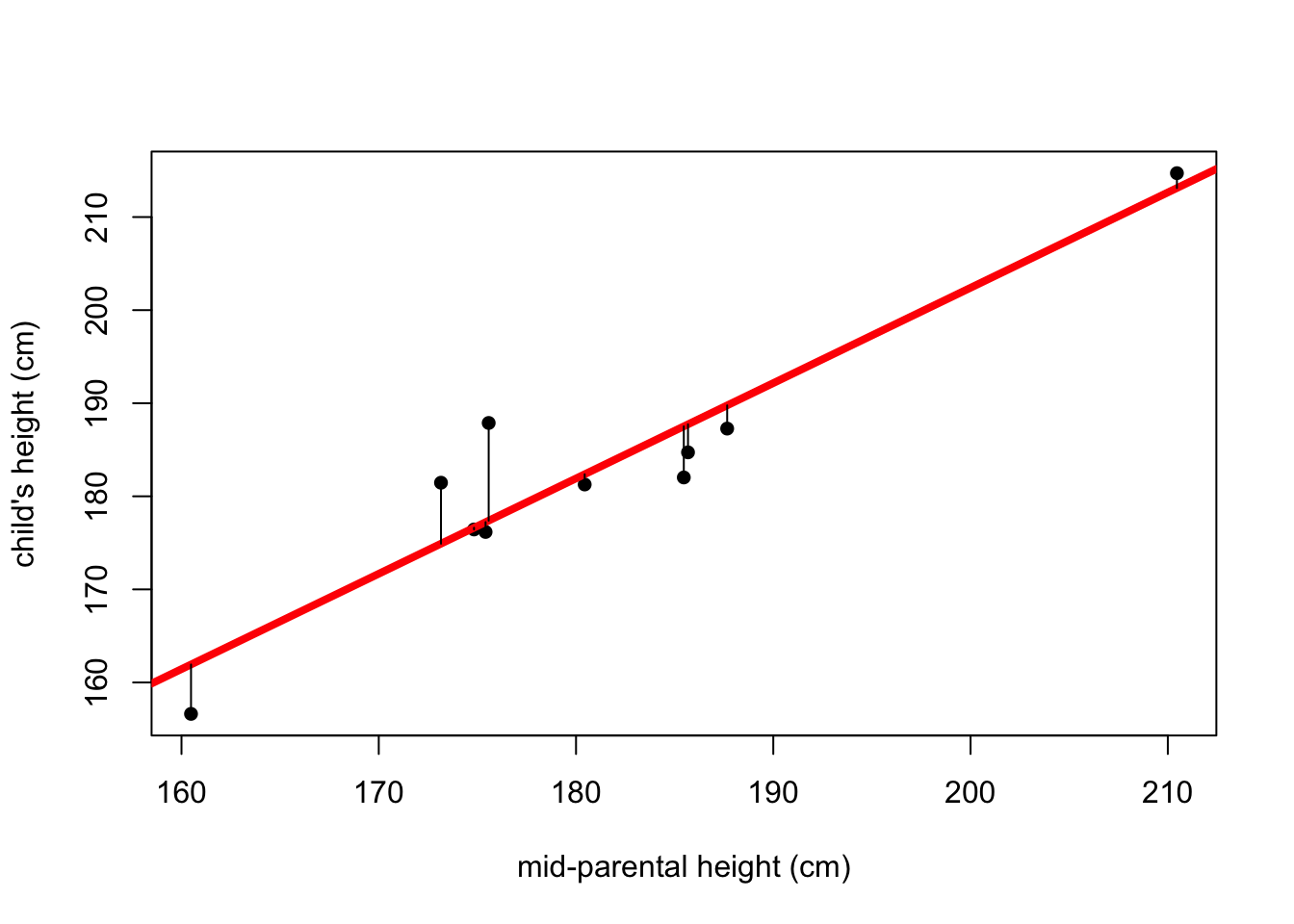
##
## Call:
## lm(formula = y ~ x)
##
## Residuals:
##    Min     1Q Median     3Q    Max
## -5.491 -2.882 -1.077  1.151 10.494
##
## Coefficients:
##             Estimate Std. Error t value Pr(>|t|)
## (Intercept)  -2.4346    24.8950  -0.098    0.925
## x             1.0242     0.1373   7.460 7.19e-05 ***
## ---
## Signif. codes:  0 '***' 0.001 '**' 0.01 '*' 0.05 '.' 0.1 ' ' 1
##
## Residual standard error: 5.38 on 8 degrees of freedom
## Multiple R-squared:  0.8743, Adjusted R-squared:  0.8586
## F-statistic: 55.66 on 1 and 8 DF,  p-value: 7.193e-05
#you need to load the MASS library to use the mvrnorm() function
library(MASS)
#generate some simulated data
#the function mvrnorm generates a matrix in which you need to specify the mean, variance and covariance
#Note that when you run this it generates random data so it will not look like what I showed in class.
xy <- mvrnorm(10,mu=c(180,180),matrix(c(100,85,85,100),2))
var(xy)## [,1] [,2]
## [1,] 86.22372 70.84882
## [2,] 70.84882 75.73134x <- xy[,1]
y <- xy[,2]
#plot the scatter points
plot(x,y, pch=16, xlab="mid-parental height (cm)", ylab="child's height (cm)")
#to perform linear regression of x against y using least squares we use the ~ symbol
lm(y~x)##
## Call:
## lm(formula = y ~ x)
##
## Coefficients:
## (Intercept) x
## 33.3041 0.8217#however, this doesn't get us a very informative output, so we use summary()
#which gives us the slope and intercept as well as the t-test and the ANOVA
summary(lm(y~x))##
## Call:
## lm(formula = y ~ x)
##
## Residuals:
## Min 1Q Median 3Q Max
## -6.3667 -2.8269 0.6699 2.4445 6.8047
##
## Coefficients:
## Estimate Std. Error t value Pr(>|t|)
## (Intercept) 33.3041 28.9606 1.150 0.283366
## x 0.8217 0.1594 5.156 0.000867 ***
## ---
## Signif. codes: 0 '***' 0.001 '**' 0.01 '*' 0.05 '.' 0.1 ' ' 1
##
## Residual standard error: 4.439 on 8 degrees of freedom
## Multiple R-squared: 0.7687, Adjusted R-squared: 0.7398
## F-statistic: 26.59 on 1 and 8 DF, p-value: 0.0008675#we can save the output of lm as a variable
linear.model <- lm(y~x)
#this saves it as a lm object
class(linear.model)## [1] "lm"#and then we can run the function confint() which returns the 95% confidence interval for the two parameters (intercept in the first row and slope in the second row).
confint(linear.model)## 2.5 % 97.5 %
## (Intercept) -33.4791096 100.087327
## x 0.4542198 1.189152#we can now predict a y value (i.e. a child's height) based on an x value (the mid-parental height) using the linear model. The first argument is the model and the second argument is the value of x. Note that we have to specify it in list form.
predict(linear.model, list(x=180))## 1
## 181.2076## 1 2 3 4
## 176.2775 181.2076 185.3160 189.4245#To add a line to the plot that shows that linear model:
abline(linear.model, col="red", lwd=4)
#This also works, and is what I typically do:
abline(lm(y~x), col="red", lwd=4)
#If we use predict() we get the values of y from the model for each of the values of x that were used to fit the model
predict(lm(y~x))## 1 2 3 4 5 6 7 8
## 181.7120 181.7247 174.3574 189.4537 182.3192 189.7933 195.4341 178.4548
## 9 10
## 181.9388 169.4279## 1 2 3 4 5 6 7 8
## 181.7120 181.7247 174.3574 189.4537 182.3192 189.7933 195.4341 178.4548
## 9 10
## 181.9388 169.4279#This little bit of code will add lines depicting the residuals
fitted <- predict(lm(y~x))
for(i in 1:10) {lines(c(x[i],x[i]),c(y[i],fitted[i]))}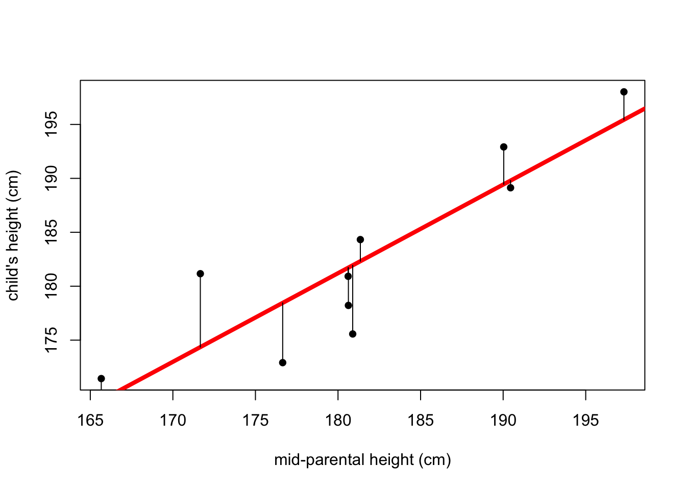
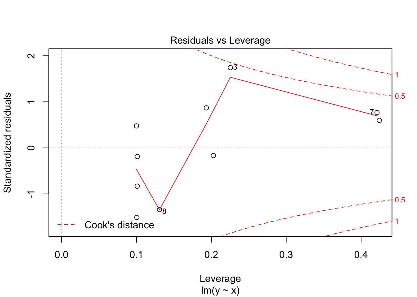
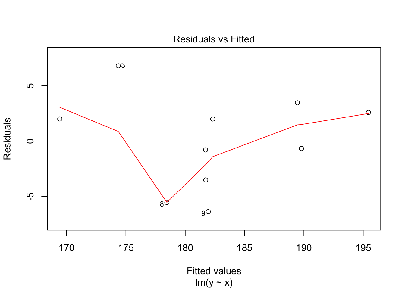
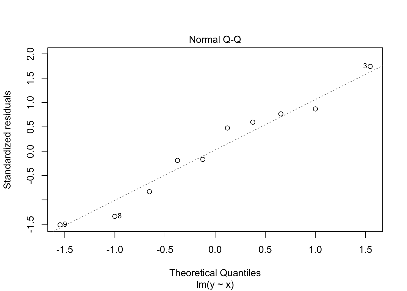
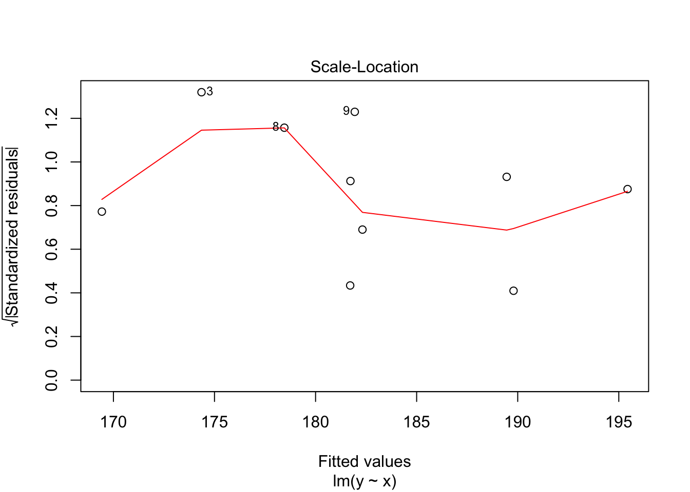
30.2 Diagnostics
Often we want to run some diagnostics on the model to assess whether our assumptions are justified e.g. whether the residuals are normally distributed or whether there are specific points that have undue influence on the model. In R there are inbuilt functions to do this. Simply use plot(lm(y~x)). This will give you four different plots with diagnostics