Chapter 11 Chi squared test
The chi-square test provides a test for the goodness of fit, where fit means how closely the observed results agree with the expected results.
The formula for the chi-square test statistic is:
11.1 Chi-squared probability densities
We can determine the probability density for the chi square distribution for 1-4 degrees of freedom using the dchisq() function
x <- 0:20
curve(dchisq(x,1),0,20, ylab="density", xlab="chi square", lwd=3, ylim=c(0,0.9))
curve(dchisq(x,2),0,20, add=T, col=2, lwd=3)
curve(dchisq(x,3),0,20, add=T, col=3, lwd=3)
curve(dchisq(x,4),0,20, add=T, col=4, lwd=3)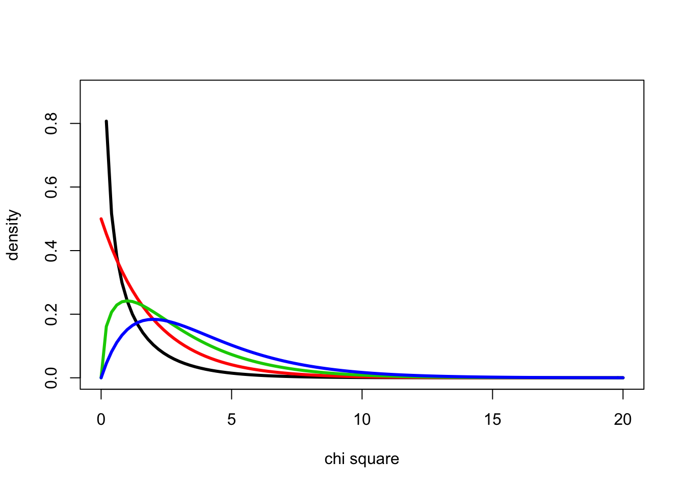
11.2 Chi-square cumulative probability distributions
We can determine the cumulative probability distributions for the chi square distribution for for 1-4 degrees of freedom using the pchisq() function
x <- 0:20
curve(pchisq(x,1),0,20, ylab="p", xlab="chi square", lwd=3)
curve(pchisq(x,2),0,20, add=T, col=2, lwd=3)
curve(pchisq(x,3),0,20, add=T, col=3, lwd=3)
curve(pchisq(x,4),0,20, add=T, col=4, lwd=3)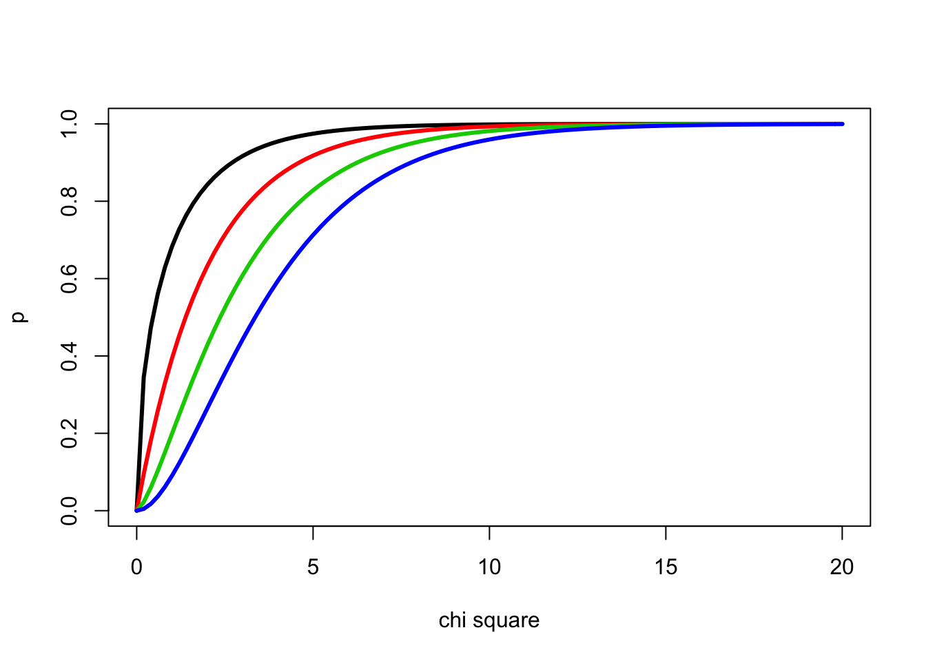
11.3 Assess results of mendel’s dihybrid cross using chi-square test statistic
# probability density for 3 degrees of freedom
x <- 0:50
curve(dchisq(x,3),0,20, ylab="density", xlab="chi square", lwd=3, ylim=c(0,0.3), col=3)

#probability density for 3 degrees of freedom; density for chisq > 0.47 indicated using polygon()
x <- 0:50
curve(dchisq(x,3),0,20, ylab="density", xlab="chi square", lwd=3, ylim=c(0,0.3), col=3)
xvals <- seq(0.47,20,length=100)
dvals <- dchisq(xvals,3)
polygon(c(xvals,rev(xvals)),c(rep(0,100),rev(dvals)), col=3)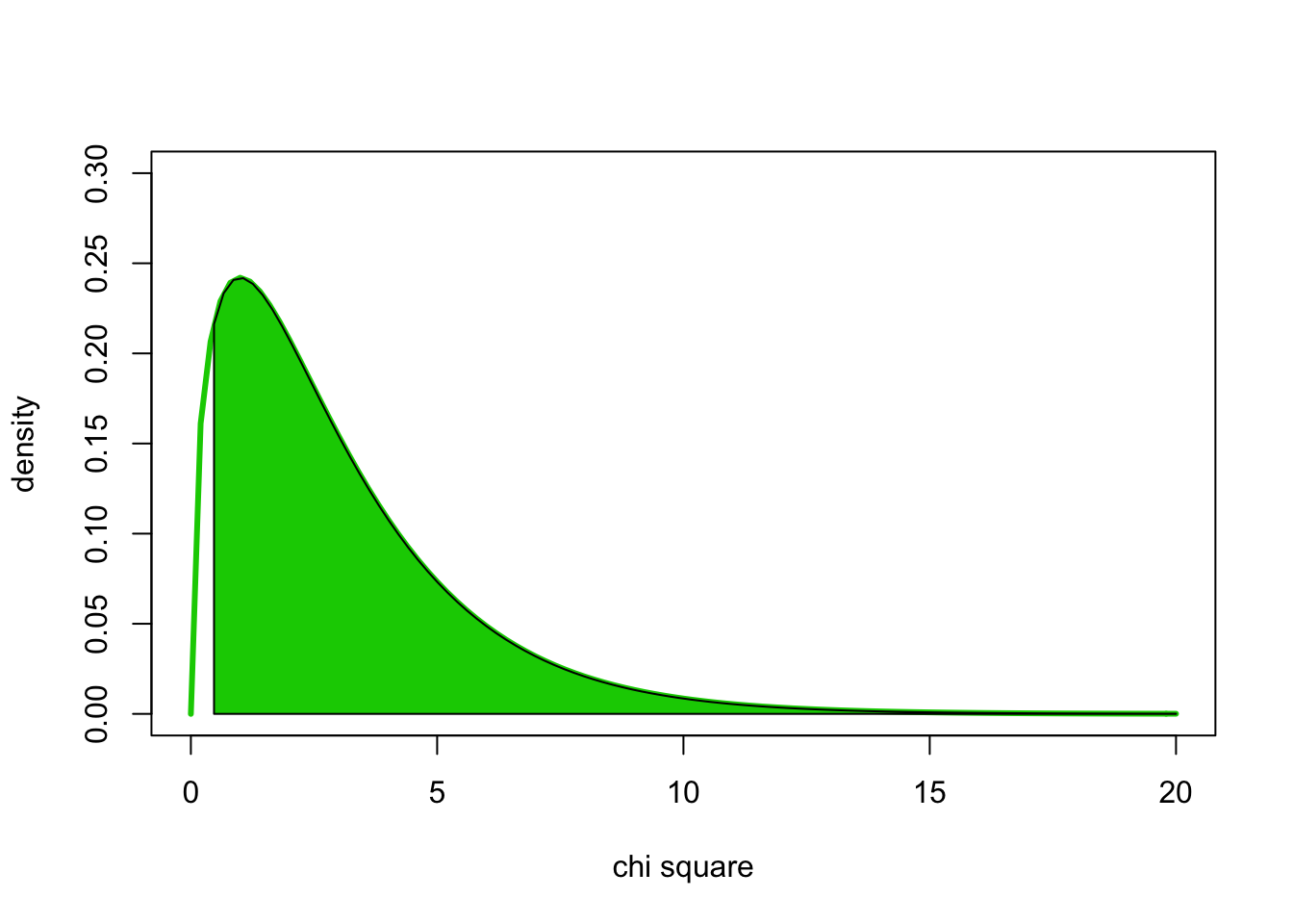
#cumulative distribution for 3 degrees of freedom with chisq=0.47 indicated using abline()
x <- 0:20
curve(pchisq(x,3),0,20, ylab="p", xlab="chi square", lwd=3, col=3)
abline(v=0.47)
abline(h=pchisq(0.47,3))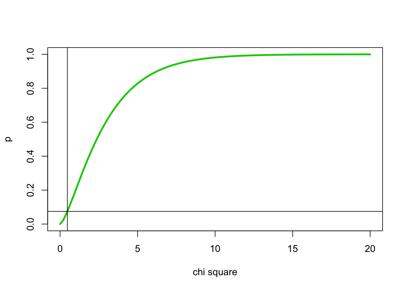
11.4 Assessing the results from the Bateson and Punnetts’s dihybrid cross using chi-square test statistic
#probability density for 1 degrees of freedom
x <- 0:50
curve(dchisq(x,1),0,50, ylab="density", xlab="chi square", lwd=3, ylim=c(0,0.5), col=1)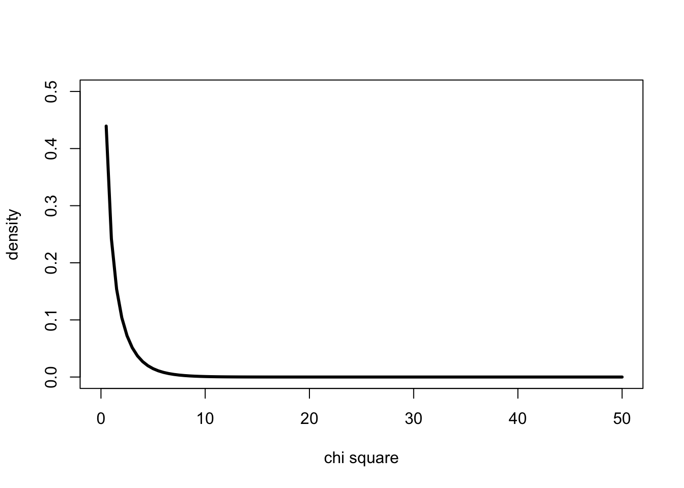
11.4.1 Log transformation
The problem is that the relevant chi square value is a very large number
one. We can do this using the log10() function
x <- 0:4000
curve(dchisq(x,1),0,log10(4000), ylab="density", xlab="log10(chi square)", lwd=3, ylim=c(0,2.2), col=1)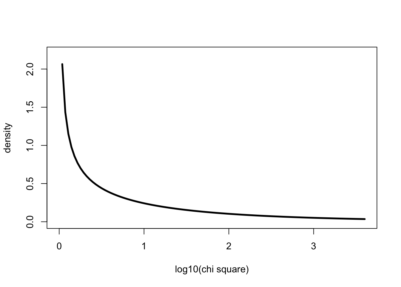
Now let’s look at the probability denisty from 3395.52 in log10 space
x <- 0:4000
curve(dchisq(x,1),0,log10(4000), ylab="density", xlab="log10(chi square)", lwd=3, ylim=c(0,2.2), col=1)
xvals <- seq(log10(3395.552),log10(4000),length=100)
dvals <- dchisq(xvals,1)
polygon(c(xvals,rev(xvals)),c(rep(0,100),rev(dvals)), col=1)
similarly, we can look at the cumulative distribution for 1 degrees of freedom with chisq=3395.552 indicated using abline()
x <- 0:4000
curve(pchisq(x,1),0,log10(4000), ylab="p", xlab="log10(chi square)", lwd=3, col=1)
abline(v=log10(3395.552))
abline(h=pchisq(log10(3395.552),1))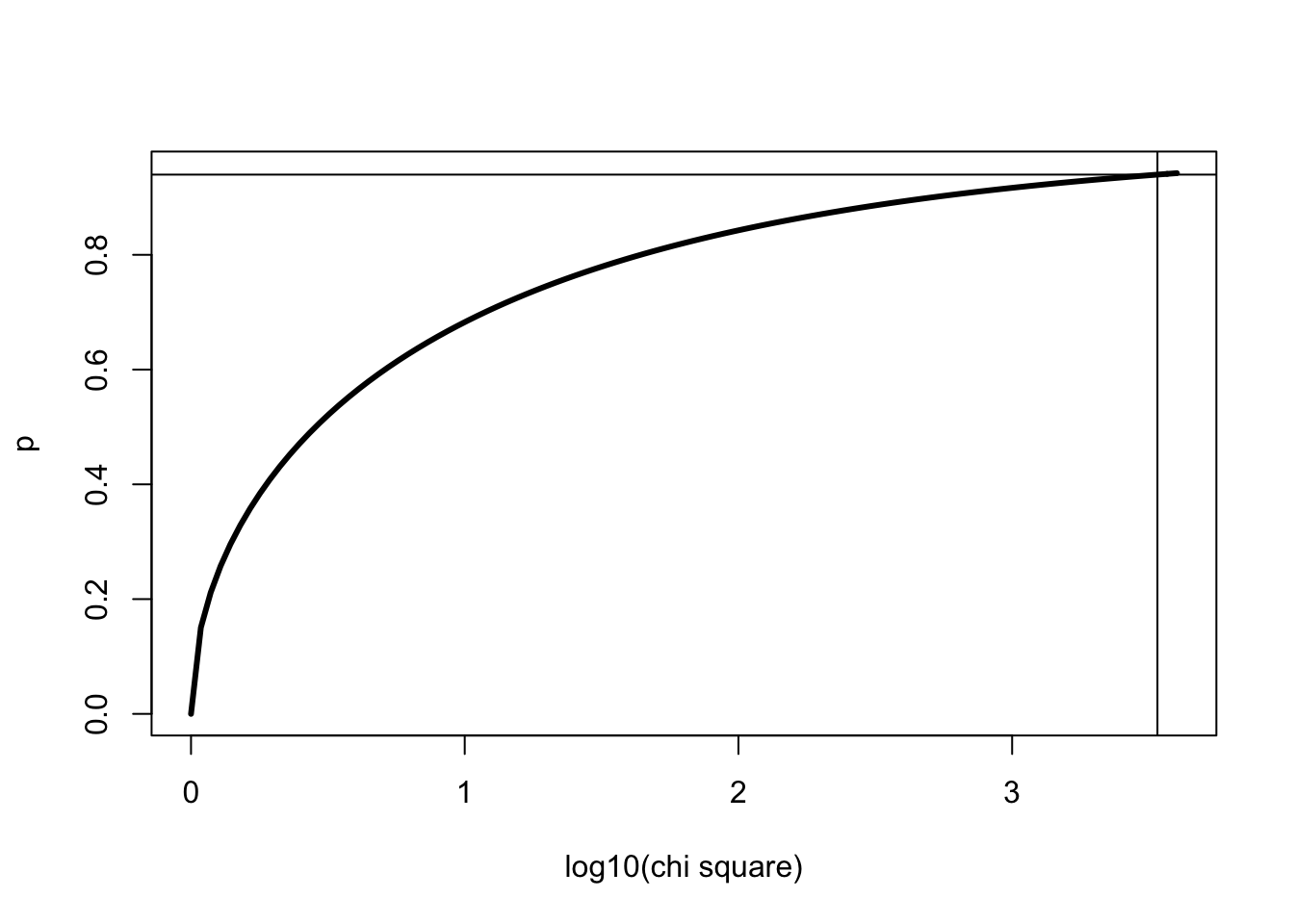
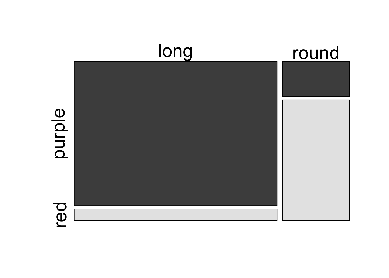
11.5 Analysis of Bateson and Punnett’s data using internal R functions
Bateson and Punnett’s data. Note that data are entered COLUMN-WISE for a matrix.
Perform chi-square test using the R function chisq.test()
##
##  Pearson's Chi-squared test
##
## data:  bp
## X-squared = 3393.6, df = 1, p-value < 2.2e-16
and, visualize the contingency table