Chapter 34 Randomization
We use randomization of a dataset to compute the null distribution of a test statistic.
#imagine that we have gene expression data for tumor and non tumor as follows
tumor <- c(20,30,25,30,20) #5 tumors
normal <- c(10,15,15,20) #4 non-tumors
#the difference between mean tumor and normal expression is:
diff <- mean(tumor) - mean(normal) #equals 10
#we can generate a null distribution for the difference between two samples of size 5 and 4 randomly drawn from the data by ignoring the labels of tumor and normal
#first concatenate the data
total <-c(tumor,normal)
#generate five random numbers between 1 and 9 (i.e. this is how we will simulate taking 5 random values from the dataset)
rand.index <- sample(1:9,5)
#the first sample of 5 we take using the randomly generated indices
rand.1 <- total[rand.index]
#the second sample is everything else
rand.2 <- total[-rand.index]
#calculate the differences in the means between the random sample of 5 and 4 valuues from the entire dataset.
diff.rand <- mean(rand.1) - mean(rand.2)
#if we put that in a loop we can use permutation to generate a null hypothesis for the difference in means
perm.results <- matrix(data=NA, nrow=10000, ncol=1)
for(i in 1:length(perm.results)){
rand.index <- sample(1:9,5)
rand.1 <- total[rand.index]
rand.2 <- total[-rand.index]
perm.results[i,1] <- mean(rand.1) - mean(rand.2)
}
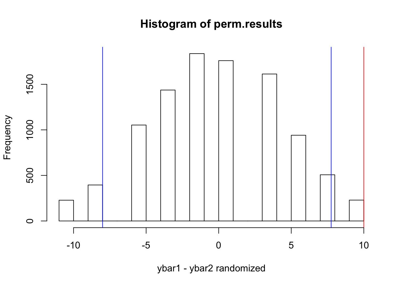
#let's look at the distribution of differences between the means of permuted (scambled data)
hist(perm.results, xlab="ybar1 - ybar2 randomized")
#add lines that define the 95% CI for the difference between the means
quantile(perm.results,probs=c(0.025,0.975)) #these are the values## 2.5% 97.5%
## -8.00 7.75abline(v=quantile(perm.results,probs=c(0.025,0.975)), col="blue")
#add a line for the actual difference in means of the tumor and normal sample
abline(v=diff,col="red") #should lie outside of the critical region