Chapter 36 Statistical Power
36.1 What is statistical power?
#Set a range of x values
x.values <- seq(-4,4,0.01)

#Plot a  distribution of t values with 3 degrees of freedom for the corresponding x values
plot(x.values,dt(x.values, 3), type="l", lty=1, lwd=2, ylim=c(0,0.4), xlab="t", ylab="probability", xlim=c(-4,10))

#add lines that define the 5% critical values for the t distribution with 3 degrees of freedom
abline(v=qt(c(0.025,0.975),3), col="black")

#Plot a  distribution of t values with 3 degrees of freedom for the corresponding x values in which the true difference is 5
lines(x.values+5,dt(x.values, 3), type="l", lty=2, lwd=2)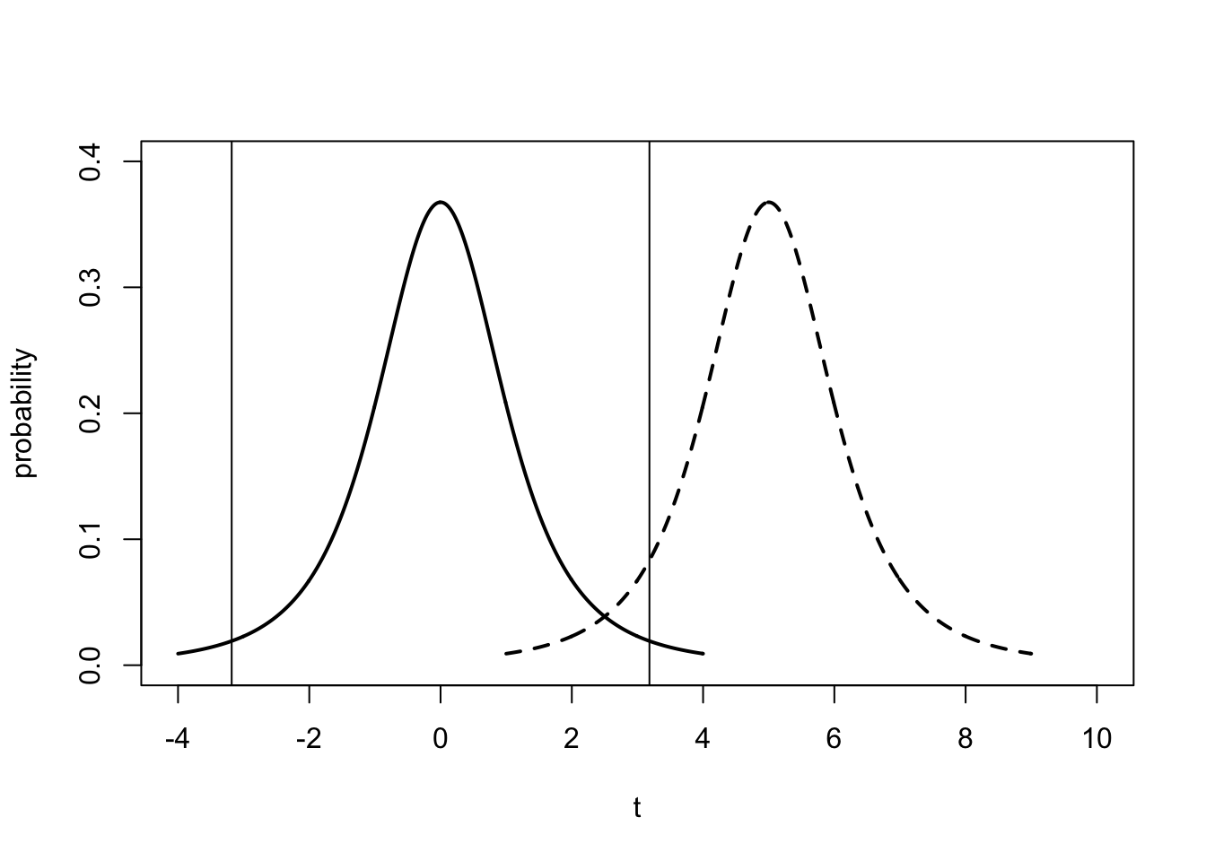
#Effect of a greater magnitude of difference
#Plot a  distribution of t values with 3 degrees of freedom for the corresponding x values
plot(x.values,dt(x.values, 3), type="l", lty=1, lwd=2, ylim=c(0,0.4), xlab="t", ylab="probability", xlim=c(-4,10))

#add lines that define the 5% critical values for the t distribution with 3 degrees of freedom
abline(v=qt(c(0.025,0.975),3), col="black")

#increase the difference between the means from 0 to 7
lines(x.values+7,dt(x.values, 3), type="l", lty=4, lwd=2)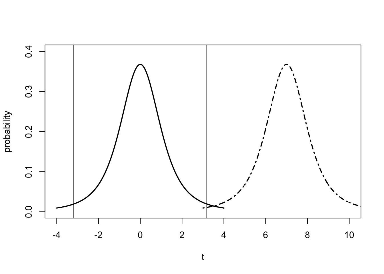
#Effect of a bigger sample size
#Plot a  distribution of t values with 3 degrees of freedom for the corresponding x values
plot(x.values,dt(x.values, 30), type="l", lty=1, lwd=2, ylim=c(0,0.4), xlab="t", ylab="probability", xlim=c(-4,10))

#add lines that define the 5% critical values for the t distribution with 3 degrees of freedom
abline(v=qt(c(0.025,0.975),30), col="black")

#Plot a  distribution of t values with 3 degrees of freedom for the corresponding x values
lines(x.values+5,dt(x.values, 30), type="l", lty=6, lwd=2)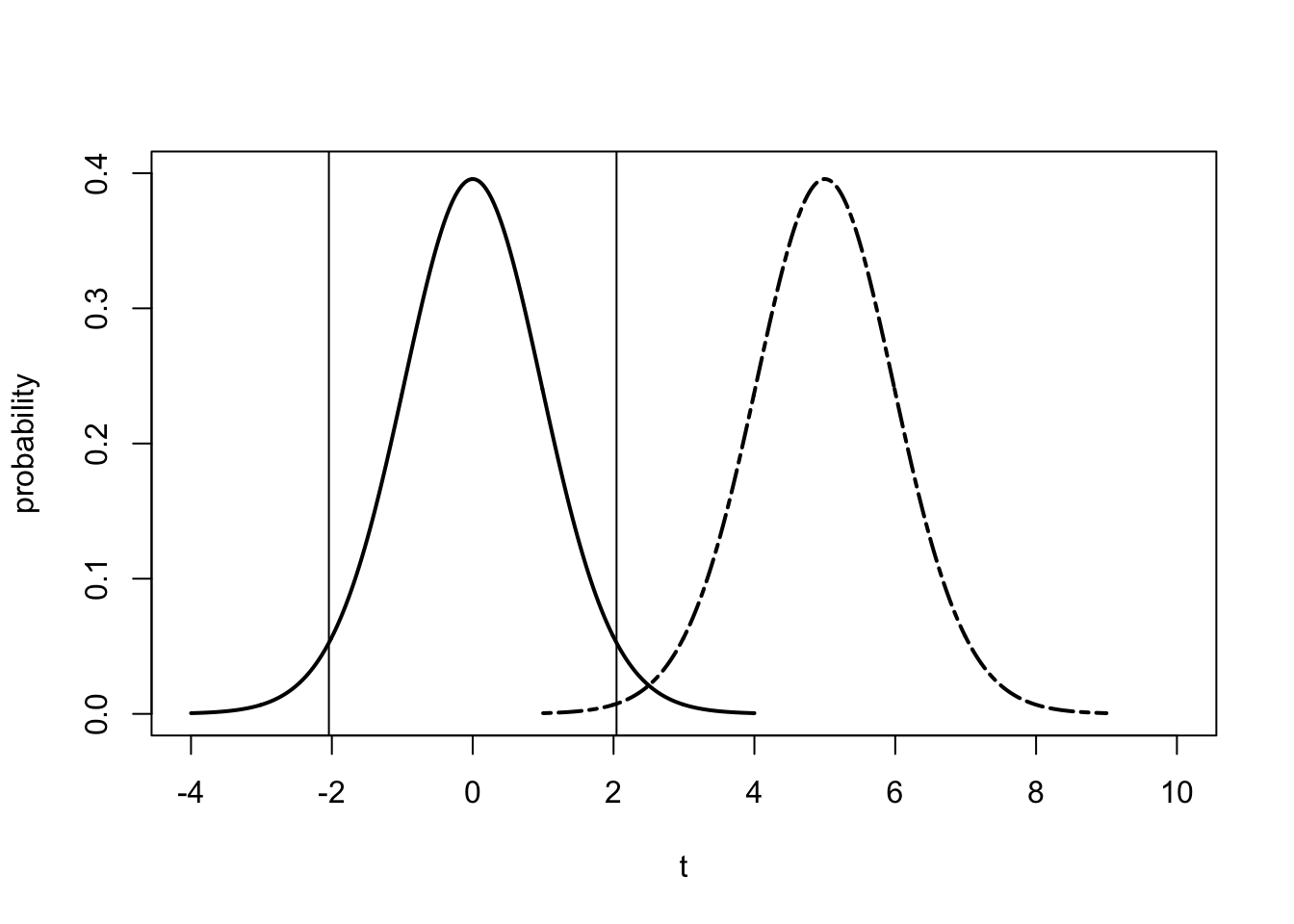
#Effect of a bigger sample size but more stringent alpha
#Plot a  distribution of t values with 3 degrees of freedom for the corresponding x values
plot(x.values,dt(x.values, 30), type="l", lty=1, lwd=2, ylim=c(0,0.4), xlab="t", ylab="probability", xlim=c(-4,10))

#add lines that define the 5% critical values for the t distribution with 3 degrees of freedom
abline(v=qt(c(0.005,0.995),30), col="black")

#Plot a  distribution of t values with 3 degrees of freedom for the corresponding x values
lines(x.values+5,dt(x.values, 30), type="l", lty=6, lwd=2)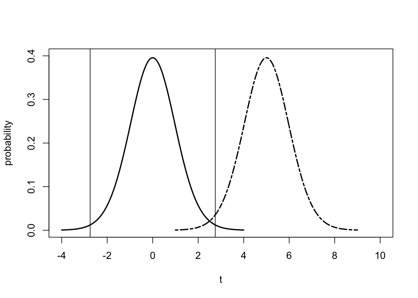
36.2 Performing Power Analysis
Required sample size for measuring a mean with a desired precision. a function to compute the required sample size for estimating a mean with a specified precision that requires a standard deviation, a half-width interval and a maximum sample size
my.pwr.test <- function(my.sd,my.d,max.n){
  n.range <- matrix(nrow=max.n, ncol=2, dimnames = as.list(c(),c("n.guess", "n.val")))
  for(i in 3:max.n) {
  n.range[i,1] <- i
  n.range[i,2] <- ((my.sd)^2*qt(0.975,i-1)^2)/my.d^2
  }

print(n.range)

#the minimum on this plot is the point of convergence for the iterative calculation
#it defines the minimal sample size required to measure the mean with the specified precision
plot(-1*log10(abs(n.range[,1]-n.range[,2])))
abline(v=which.min(abs(n.range[,1]-n.range[,2])), lty=2, lwd=3, col=2)

#print out the minimum sample size required
print("minimum sample size required:")
print(which.min(abs(n.range[,1]-n.range[,2])))

}

#example
my.pwr.test(30,10,40)
## [,1] [,2]
## [1,] NA NA
## [2,] NA NA
## [3,] 3 166.61538
## [4,] 4 91.15168
## [5,] 5 69.37783
## [6,] 6 59.47102
## [7,] 7 53.88640
## [8,] 8 50.32303
## [9,] 9 47.85890
## [10,] 10 46.05620
## [11,] 11 44.68142
## [12,] 12 43.59902
## [13,] 13 42.72503
## [14,] 14 42.00473
## [15,] 15 41.40099
## [16,] 16 40.88769
## [17,] 17 40.44599
## [18,] 18 40.06190
## [19,] 19 39.72486
## [20,] 20 39.42675
## [21,] 21 39.16119
## [22,] 22 38.92314
## [23,] 23 38.70855
## [24,] 24 38.51410
## [25,] 25 38.33710
## [26,] 26 38.17529
## [27,] 27 38.02681
## [28,] 28 37.89008
## [29,] 29 37.76375
## [30,] 30 37.64668
## [31,] 31 37.53789
## [32,] 32 37.43654
## [33,] 33 37.34188
## [34,] 34 37.25327
## [35,] 35 37.17016
## [36,] 36 37.09204
## [37,] 37 37.01849
## [38,] 38 36.94910
## [39,] 39 36.88355
## [40,] 40 36.82151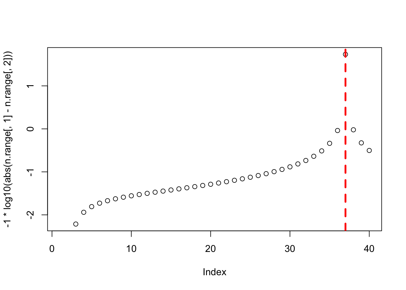
## [1] "minimum sample size required:"
## [1] 37