Chapter 4 An introduction to R
In order to use statistics we need to learn how to writing small computer “programs”, which are simply lists of commands that we tell a computer to execute.
Luckily for us, there is a computer programming language that is written specifically for this purpose. This language has the very imaginative name, R. The great thing about R is that it is entirely free and a large community works with it creating resources and tools that can be used by all of us.
4.1 Installing R and Rstudio
Before we proceed we need to get a copy of R on our computer. That can be done simply by downloading the program and following the installation instructions here.
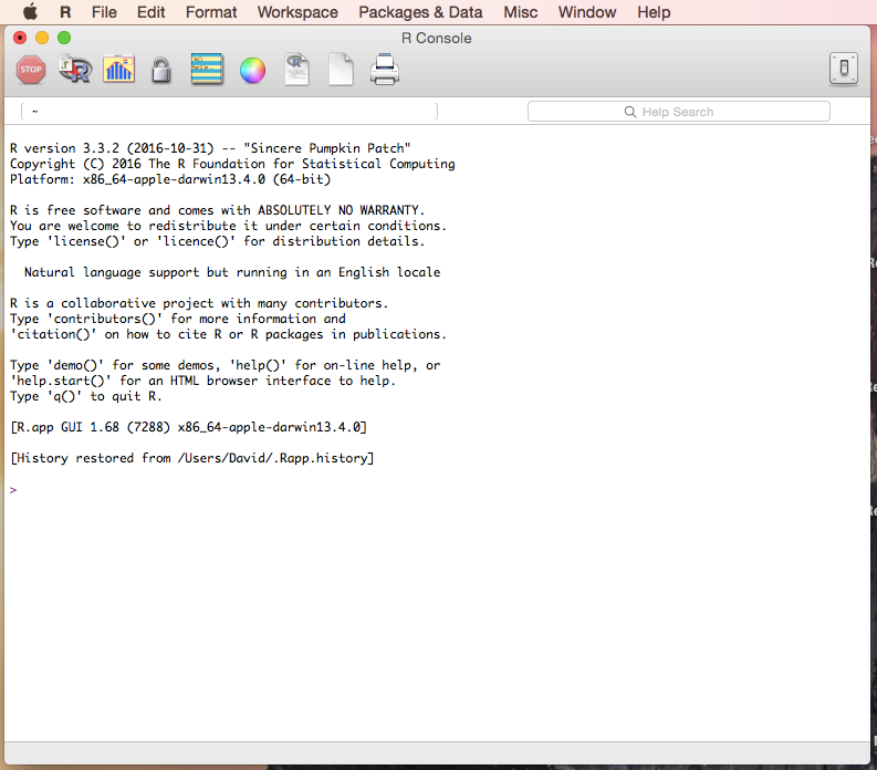
Once you have R installed you can open it up and see something that looks like this:
Straight away, I am going to suggest using something different that will ultimately make your R experience, and therefore your whole life, much more enjoyable. That is RStudio, an integrated development environment (IDE). Essentially all that it is a souped up R console in which you can organize multiple windows to work seamlessly with R. Trust me.
Go get yourself a free copy here.
Once you have installed that it should look liked this:
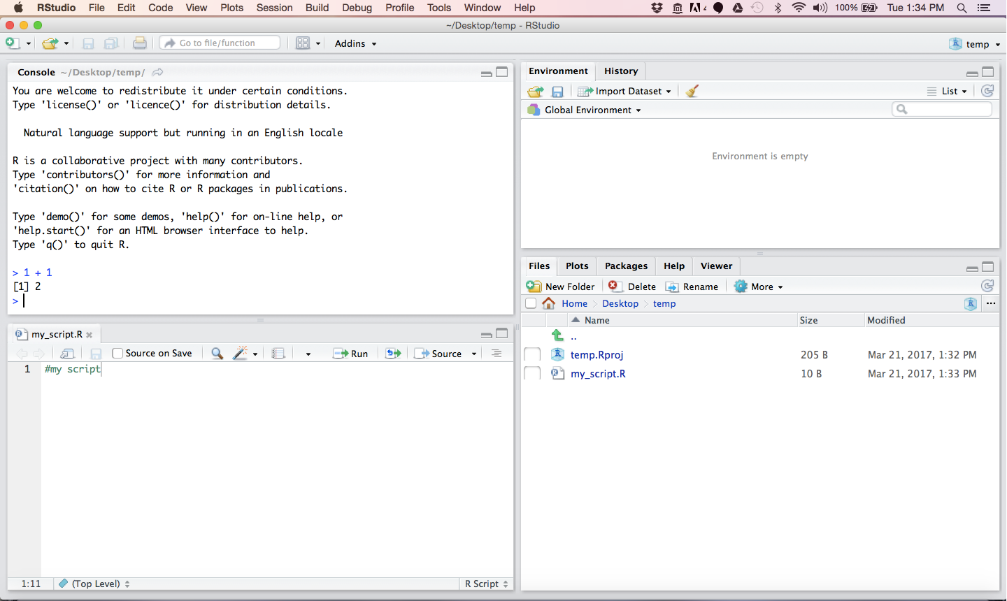
And now we are in bussiness
4.2 Using R as a calculator
It is useful to think of R as a calculator in which we can do normal calculations.
Try the following in which we so simple arithmetic such as:
\(10 + 10 = 20\)
## [1] 20or \(10 * 10 = 100\):
## [1] 100or any other basic calculation we want to do:
## [1] 1## [1] 0## [1] 100## [1] 2.302585as you can see R executes each of the commands and returns an anwswer
4.3 Using variables
One thing that you will want to do is store the answer so that you can use that again. The way that we do that is by assigning the result using the synatx x <- 10. If we do this we can then use the symbol x for our calculations.
## [1] 10## [1] 20## [1] 100## [1] 1## [1] 0## [1] 100## [1] 2.302585This becomes really useful because now we could go back and change x to 100 using x <- 100 and redo all the calculations without having to write everything out again.
4.4 Bring some external data into R
Oftentimes we’ll have some data in a table and want to bring those data into R. That’s easy:
##         Name Height.cm
## 1   Student1    168.00
## 2   Student2    165.00
## 3   Student3    173.00
## 4   Student4    168.00
## 5   Student5    173.00
## 6   Student6    171.00
## 7   Student7    168.00
## 8   Student8    165.00
## 9   Student9    166.00
## 10 Student10    173.00
## 11 Student11    163.00
## 12 Student12    164.00
## 13 Student13    178.00
## 14 Student14    163.00
## 15 Student15    178.00
## 16 Student16    167.64
## 17 Student17    188.00
These data are stored in something called a dataframe. In this case the dataframe has two columns and in order to access the data in the second colummn we need to explcitly use its column name with the syntax class.heights$Height.cm
##  [1] 168.00 165.00 173.00 168.00 173.00 171.00 168.00 165.00 166.00 173.00
## [11] 163.00 164.00 178.00 163.00 178.00 167.64 188.00
4.5 Analyze the data
You are probably already familiar with some statistical concepts. Even if you aren’t you can see how we can work with these data using in built functions in R.
## [1] 170.0965## [1] 163## [1] 188## [1] 163 188## [1] 168## [1] 43.58821## [1] 6.6021374.6 Making a plot
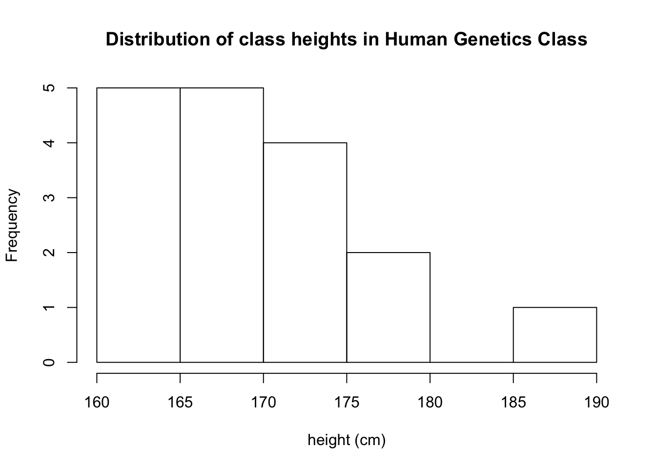
As humans are very visual animals, seeing the data is the best way to get a feel for the data. R is great at this.
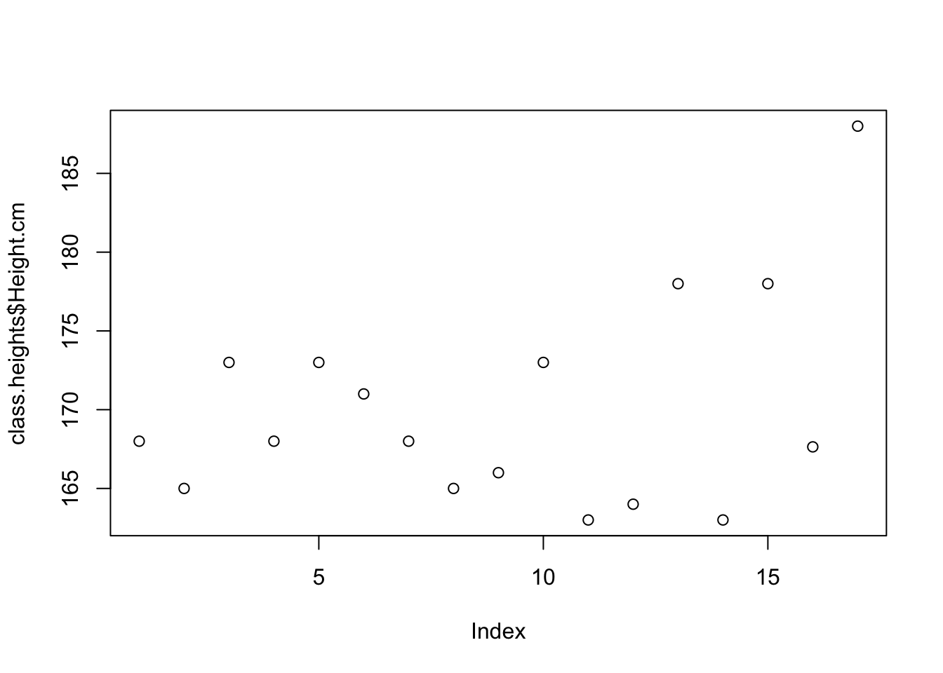
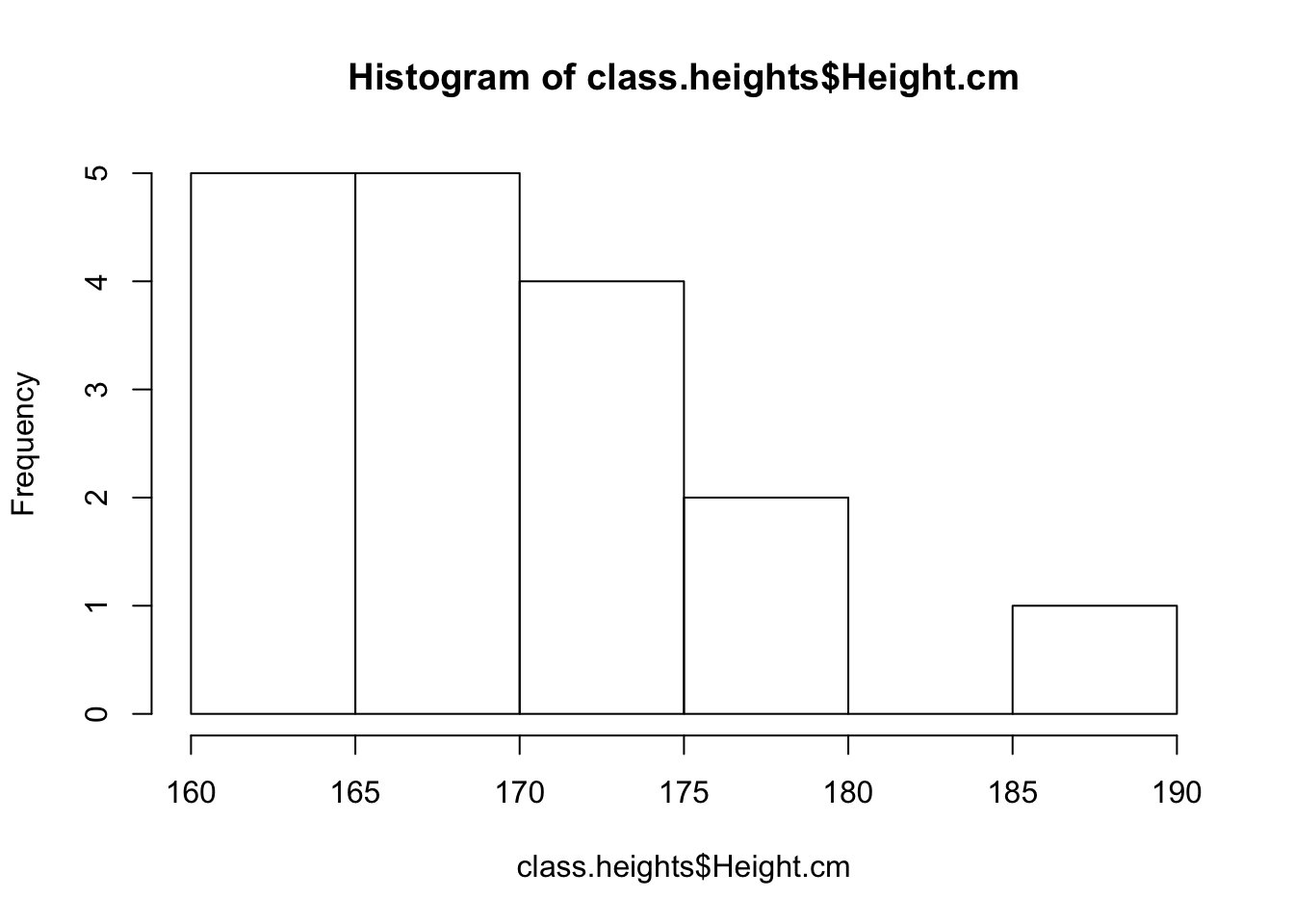
Clearly, a histogram is a much better way of depicting the data.
4.7 Saving the plot and saving everything
With a little bit of work we can make the plot look very nice.
4.8 Keeping a record of everything using R markdown.
When you start working with R a lot you’ll quickly find that you have many files and many graphs and you’ll lose track of how things were done. The solution to this is to keep everything in a single file. We do that using an R Markdown file. The procedure is simple:
- In Rstudio we open a new file using
File -> New File -> R Mardown…
- We write our code in chunks using
Insert -> R
in the pull down menu
- When we have completed our code we run:
Knit to HTML
which generated a nice record of everything with the R code and the results of running the R code in one place.
In fact, R Markdown is so useful I wrote this book using this method.