Chapter 35 Bootstrapping
Bootstrapping allows us to estimate the precision with which we can estimate the mean of a sample by using the sample as a “population” and resampling from it with replacement to generate the sampling distribution of the mean
Imagine that we have a sample of 10 values from our mRNA.count data (from the simulation section)
#To simulate this, generate a population of 1100 cells that have 10 or 11 or 12...or 20 mRNAs per cell
mRNA.count <- c(rep(10,100),rep(11,100),rep(12,100),rep(13,100),rep(14,100),
                rep(15,100),rep(16,100),rep(17,100),rep(18,100),rep(19,100),
                rep(20,100))

my.sample <- sample(mRNA.count, 10)

#The mean of this sample is:
mean(my.sample)
## [1] 15.1#We could estimate the standard error of the mean using our standard method
#But, bootstrapping allows us to do this by resampling the sample WITH replacement and estimating the sampling distribution of the mean. The same sample size should be used.
new.sample <- sample(my.sample,10,replace=T)
mean(new.sample)## [1] 13.9#we can do this many times using a loop
perm.sample <- matrix(data=NA, nrow=10000, ncol=1)
for(i in 1:length(perm.sample)){
new.sample <- sample(my.sample,10,replace=T)
perm.sample[i,1] <- mean(new.sample)
}
#plot the distribution of means
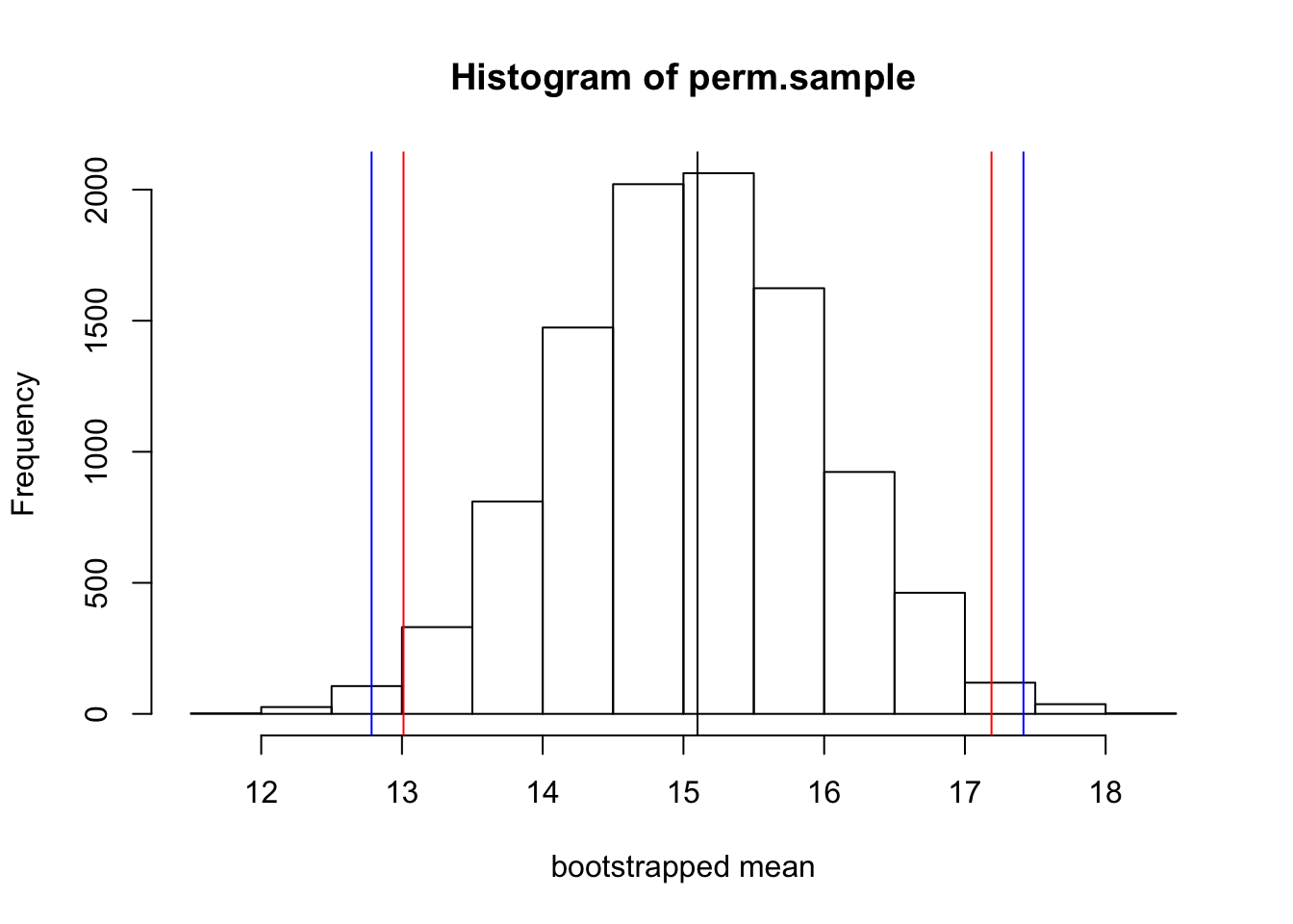
hist(perm.sample, xlab="bootstrapped mean") #this is analagous to the sampling distribution of means
#Therefore the sd of this distribution is analagous to our standard error of the mean
sd(perm.sample)## [1] 0.9233917## [1] 0.9712535#we can compute the 95%CI of the mean using the sd of the permuted means rather than the standard error of the mean of our sample
abline(v=mean(my.sample))
abline(v=mean(my.sample)+sd(perm.sample)*qt(0.025,9), col="red")
abline(v=mean(my.sample)+sd(perm.sample)*qt(0.975,9), col="red")
#let's compare this to the values estimated from the standard error of the mean
abline(v=mean(my.sample)+sd(my.sample)/sqrt(9)*qt(0.025,9), col="blue")
abline(v=mean(my.sample)+sd(my.sample)/sqrt(9)*qt(0.975,9), col="blue")